


datamatrix.series
- What are series?
- function baseline(series, baseline, bl_start=-100, bl_end=None, reduce_fnc=None, method=u'subtractive')
- function blinkreconstruct(series, vt=5, vt_start=10, vt_end=5, maxdur=500, margin=10, smooth_winlen=21, std_thr=3, gap_margin=20, gap_vt=10, mode=u'original')
- function concatenate(*series)
- function downsample(series, by, fnc=)
- function endlock(series)
- function fft(series, truncate=True)
- function filter_bandpass(series, freq_range, order=2, sampling_freq=None)
- function filter_highpass(series, freq_min, order=2, sampling_freq=None)
- function filter_lowpass(series, freq_max, order=2, sampling_freq=None)
- function interpolate(series)
- function lock(series, lock)
- function normalize_time(dataseries, timeseries)
- function reduce(series, operation=)
- function reduce(series, operation=)
- function smooth(series, winlen=11, wintype=u'hanning')
- function threshold(series, fnc, min_length=1)
- function window(series, start=0, end=None)
- function z(series)
What are series?
A SeriesColumn is a column with a depth; that is, each cell contains multiple values. Data of this kind is very common. For example, imagine a psychology experiment in which participants see positive or negative pictures, while their brain activity is recorded using electroencephalography (EEG). Here, picture type (positive or negative) is a single value that could be stored in a normal table. But EEG activity is a continuous signal, and could be stored as SeriesColumn.
For more information, see:
function baseline(series, baseline, bl_start=-100, bl_end=None, reduce_fnc=None, method=u'subtractive')
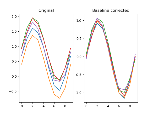
Applies a baseline to a signal
Example:
import numpy as np
from matplotlib import pyplot as plt
from datamatrix import DataMatrix, SeriesColumn, series as srs

LENGTH = 5 # Number of rows
DEPTH = 10 # Depth (or length) of SeriesColumns

sinewave = np.sin(np.linspace(0, 2*np.pi, DEPTH))

dm = DataMatrix(length=LENGTH)
# First create five identical rows with a sinewave
dm.y = SeriesColumn(depth=DEPTH)
dm.y.setallrows(sinewave)
# Add a random offset to the Y values
dm.y += np.random.random(LENGTH)
# And also a bit of random jitter
dm.y += .2*np.random.random( (LENGTH, DEPTH) )
# Baseline-correct the traces, This will remove the vertical
# offset
dm.y2 = srs.baseline(dm.y, dm.y, bl_start=0, bl_end=10)

plt.clf()
plt.subplot(121)
plt.title('Original')
plt.plot(dm.y.plottable)
plt.subplot(122)
plt.title('Baseline corrected')
plt.plot(dm.y2.plottable)
plt.show()
Arguments:
series-- The signal to apply a baseline to.- Type: SeriesColumn
baseline-- The signal to use as a baseline to.- Type: SeriesColumn
Keywords:
bl_start-- The start of the window frombaselineto use.- Type: int
- Default: -100
bl_end-- The end of the window frombaselineto use, or None to go to the end.- Type: int, None
- Default: None
reduce_fnc-- The function to reduce the baseline epoch to a single value. If None, np.nanmedian() is used.- Type: FunctionType, None
- Default: None
method-- Specifies whether divisive or subtractive baseline correction should be used. (Changed in v0.7.0: subtractive is now the default)- Type: str
- Default: 'subtractive'
Returns:
A baseline-correct version of the signal.
- Type: SeriesColumn
function blinkreconstruct(series, vt=5, vt_start=10, vt_end=5, maxdur=500, margin=10, smooth_winlen=21, std_thr=3, gap_margin=20, gap_vt=10, mode=u'original')
Reconstructs pupil size during blinks. This algorithm has been designed and tested largely with the EyeLink 1000 eye tracker.
Version note: As of 0.13.0, an advanced algorithm has been
introduced, wich can be specified through the mode keyword. The
advanced algorithm is recommended for new analyses, and will be made
the default in future releases.
Source:
- Mathot, S. (2013). A simple way to reconstruct pupil size during eye blinks. http://doi.org/10.6084/m9.figshare.688002
Arguments:
series-- A signal to reconstruct.- Type: SeriesColumn
Keywords:
vt-- A pupil-velocity threshold for blink detection. Lower tresholds more easily trigger blinks. This argument only applies to 'original' mode.- Type: int, float
- Default: 5
vt_start-- A pupil-velocity threshold for detecting the onset of a blink. Lower tresholds more easily trigger blinks. This argument only applies to 'advanced' mode.- Type: int, float
- Default: 10
vt_end-- A pupil-velocity threshold for detecting the offset of a blink. Lower tresholds more easily trigger blinks. This argument only applies to 'advanced' mode.- Type: int, float
- Default: 5
maxdur-- The maximum duration (in samples) for a blink. Longer blinks are not reconstructed.- Type: int
- Default: 500
margin-- The margin to take around missing data that is reconstructed.- Type: int
- Default: 10
smooth_winlen-- The window length for a hanning window that is used to smooth the velocity profile.- Type: int
- Default: 21
std_thr-- A standard-deviation threshold for when data should be considered invalid.- Type: float, int
- Default: 3
gap_margin-- The margin to take around missing data that is not reconstructed. Only applies to advanced mode.- Type: int
- Default: 20
gap_vt-- A pupil-velocity threshold for detection of invalid data. Lower tresholds mean more data marked as invalid. Only applies to advanced mode.- Type: int, float
- Default: 10
mode-- The algorithm to be used for blink reconstruction. Should be 'original' or 'advanced'. An advanced algorith was introduced in v0.13., and should be used for new analysis. The original algorithm is still the default for backwards compatibility.- Type: str
- Default: 'original'
Returns:
A reconstructed singal.
- Type: SeriesColumn
function concatenate(*series)
Concatenates multiple series such that a new series is created with a depth that is equal to the sum of the depths of all input series.
Example:
from datamatrix import series as srs

dm = DataMatrix(length=1)
dm.s1 = SeriesColumn(depth=3)
dm.s1[:] = 1,2,3
dm.s2 = SeriesColumn(depth=3)
dm.s2[:] = 3,2,1
dm.s = srs.concatenate(dm.s1, dm.s2)
print(dm.s)
Output:
col[[1. 2. 3. 3. 2. 1.]]
Argument list:
*series: A list of series.
Returns:
A new series.
- Type: SeriesColumn
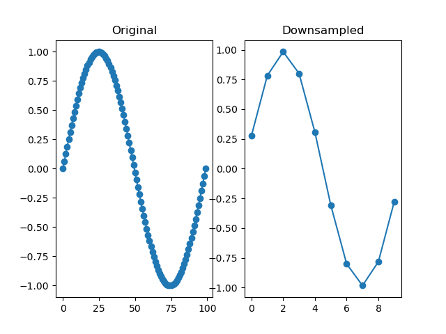
function downsample(series, by, fnc=)
Downsamples a series by a factor, so that it becomes 'by' times shorter. The depth of the downsampled series is the highest multiple of the depth of the original series divided by 'by'. For example, downsampling a series with a depth of 10 by 3 results in a depth of 3.
Example:
import numpy as np
from matplotlib import pyplot as plt
from datamatrix import DataMatrix, SeriesColumn, series as srs

LENGTH = 1 # Number of rows
DEPTH = 100 # Depth (or length) of SeriesColumns

sinewave = np.sin(np.linspace(0, 2*np.pi, DEPTH))

dm = DataMatrix(length=LENGTH)
dm.y = SeriesColumn(depth=DEPTH)
dm.y.setallrows(sinewave)
dm.y2 = srs.downsample(dm.y, by=10)

plt.clf()
plt.subplot(121)
plt.title('Original')
plt.plot(dm.y.plottable, 'o-')
plt.subplot(122)
plt.title('Downsampled')
plt.plot(dm.y2.plottable, 'o-')
plt.show()
Arguments:
series-- No descriptionby-- The downsampling factor.- Type: int
Keywords:
fnc-- The function to average the samples that are combined into 1 value. Typically an average or a median.- Type: callable
- Default:
Returns:
A downsampled series.
- Type: SeriesColumn
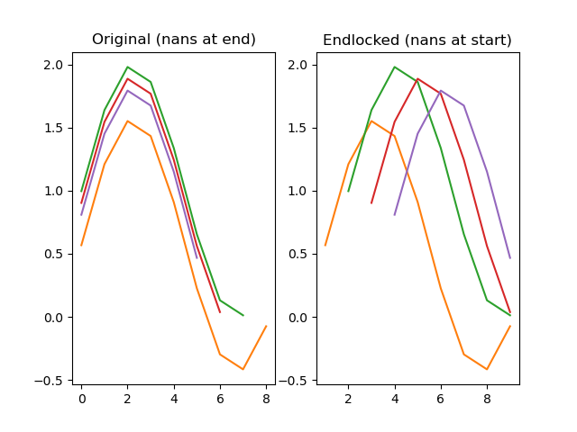
function endlock(series)
Locks a series to the end, so that any nan-values that were at the end are moved to the start.
Example:
import numpy as np
from matplotlib import pyplot as plt
from datamatrix import DataMatrix, SeriesColumn, series as srs

LENGTH = 5 # Number of rows
DEPTH = 10 # Depth (or length) of SeriesColumns

sinewave = np.sin(np.linspace(0, 2*np.pi, DEPTH))

dm = DataMatrix(length=LENGTH)
# First create five identical rows with a sinewave
dm.y = SeriesColumn(depth=DEPTH)
dm.y.setallrows(sinewave)
# Add a random offset to the Y values
dm.y += np.random.random(LENGTH)
# Set some observations at the end to nan
for i, row in enumerate(dm):
   row.y[-i:] = np.nan
# Lock the degraded traces to the end, so that all nans
# now come at the start of the trace
dm.y2 = srs.endlock(dm.y)

plt.clf()
plt.subplot(121)
plt.title('Original (nans at end)')
plt.plot(dm.y.plottable)
plt.subplot(122)
plt.title('Endlocked (nans at start)')
plt.plot(dm.y2.plottable)
plt.show()
Arguments:
series-- The signal to end-lock.- Type: SeriesColumn
Returns:
An end-locked signal.
- Type: SeriesColumn
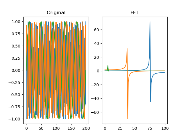
function fft(series, truncate=True)
New in v0.9.2
Performs a fast-fourrier transform (FFT) for the signal. For more
information, see numpy.fft.
Example:
import numpy as np
from matplotlib import pyplot as plt
from datamatrix import DataMatrix, SeriesColumn, series as srs

LENGTH = 3
DEPTH = 200

# Create one fast oscillation, and two combined fast and slow
# oscillations
dm = DataMatrix(length=LENGTH)
dm.s = SeriesColumn(depth=DEPTH)
dm.s[0] = np.sin(np.linspace(0, 150 * np.pi, DEPTH))
dm.s[1] = np.sin(np.linspace(0, 75 * np.pi, DEPTH))
dm.s[2] = np.sin(np.linspace(0, 10 * np.pi, DEPTH))
dm.f = srs.fft(dm.s)

# Plot the original signal
plt.clf()
plt.subplot(121)
plt.title('Original')
plt.plot(dm.s[0])
plt.plot(dm.s[1])
plt.plot(dm.s[2])
plt.subplot(122)
# And the filtered signal!
plt.title('FFT')
plt.plot(dm.f[0])
plt.plot(dm.f[1])
plt.plot(dm.f[2])
plt.show()
Arguments:
series-- A signal to determine the FFT for.- Type: SeriesColumn
Keywords:
truncate-- FFT series of real signals are symmetric. Thetruncatekeyword indicates whether the last (symmetric) part of the FFT should be removed.- Type: bool
- Default: True
Returns:
The FFT of the signal.
- Type: SeriesColumn
function filter_bandpass(series, freq_range, order=2, sampling_freq=None)
New in v0.9.2
Changed in v0.11.0: added sampling_freq argument
Applies a Butterworth bandpass-pass filter to the signal.
For more information, see scipy.signal.
Example:
import numpy as np
from matplotlib import pyplot as plt
from datamatrix import DataMatrix, SeriesColumn, series as srs

LENGTH = 3
DEPTH = 100
SAMPLING_FREQ = 100

# Create one fast oscillation, and two combined fast and slow
# oscillations
dm = DataMatrix(length=LENGTH)
dm.s = SeriesColumn(depth=DEPTH)
dm.s[0] = np.sin(np.linspace(0, 20 * np.pi, DEPTH))  # 10 Hz
dm.s[1] = np.sin(np.linspace(0, 10 * np.pi, DEPTH)) + dm.s[0]  # 5 Hz
dm.s[2] = np.cos(np.linspace(0, 2 * np.pi, DEPTH)) + dm.s[0]  # 1 Hz
dm.f = srs.filter_bandpass(dm.s, freq_range=(4, 6), sampling_freq=SAMPLING_FREQ)

# Plot the original signal
plt.clf()
plt.subplot(121)
plt.title('Original')
plt.plot(dm.s[0])
plt.plot(dm.s[1])
plt.plot(dm.s[2])
plt.subplot(122)
# And the filtered signal!
plt.title('Bandpass')
plt.plot(dm.f[0])
plt.plot(dm.f[1])
plt.plot(dm.f[2])
plt.show()
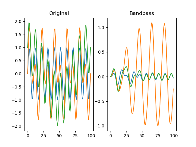
Arguments:
series-- A signal to filter.- Type: SeriesColumn
freq_range-- A(min_freq, max_freq)tuple.- Type: tuple
Keywords:
order-- The order of the filter.- Type: int
- Default: 2
sampling_freq-- The sampling frequence of the signal, orNoneto use the scipy default of 2 half-cycles per sample.- Type: int, None
- Default: None
Returns:
The filtered signal.
- Type: SeriesColumn
function filter_highpass(series, freq_min, order=2, sampling_freq=None)
New in v0.9.2
Changed in v0.11.0: added sampling_freq argument
Applies a Butterworth highpass-pass filter to the signal.
For more information, see scipy.signal.
Example:
import numpy as np
from matplotlib import pyplot as plt
from datamatrix import DataMatrix, SeriesColumn, series as srs

LENGTH = 3
DEPTH = 100
SAMPLING_FREQ = 100

# Create one fast oscillation, and two combined fast and slow
# oscillations
dm = DataMatrix(length=LENGTH)
dm.s = SeriesColumn(depth=DEPTH)
dm.s[0] = np.sin(np.linspace(0, 20 * np.pi, DEPTH))  # 10 Hz
dm.s[1] = np.sin(np.linspace(0, 2 * np.pi, DEPTH)) + dm.s[0]  # 1 Hz
dm.s[2] = np.cos(np.linspace(0, 2 * np.pi, DEPTH)) + dm.s[0]  # 1 Hz
dm.f = srs.filter_highpass(dm.s, freq_min=3, sampling_freq=SAMPLING_FREQ)

# Plot the original signal
plt.clf()
plt.subplot(121)
plt.title('Original')
plt.plot(dm.s[0])
plt.plot(dm.s[1])
plt.plot(dm.s[2])
plt.subplot(122)
# And the filtered signal!
plt.title('Highpass')
plt.plot(dm.f[0])
plt.plot(dm.f[1])
plt.plot(dm.f[2])
plt.show()
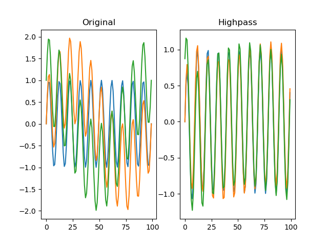
Arguments:
series-- A signal to filter.- Type: SeriesColumn
freq_min-- The minimum filter frequency.- Type: int
Keywords:
order-- The order of the filter.- Type: int
- Default: 2
sampling_freq-- The sampling frequence of the signal, orNoneto use the scipy default of 2 half-cycles per sample.- Type: int, None
- Default: None
Returns:
The filtered signal.
- Type: SeriesColumn
function filter_lowpass(series, freq_max, order=2, sampling_freq=None)
New in v0.9.2
Changed in v0.11.0: added sampling_freq argument
Applies a Butterworth low-pass filter to the signal.
For more information, see scipy.signal.
Example:
import numpy as np
from matplotlib import pyplot as plt
from datamatrix import DataMatrix, SeriesColumn, series as srs

LENGTH = 3
DEPTH = 100
SAMPLING_FREQ = 100

# Create one fast oscillation, and two combined fast and slow
# oscillations
dm = DataMatrix(length=LENGTH)
dm.s = SeriesColumn(depth=DEPTH)
dm.s[0] = np.sin(np.linspace(0, 20 * np.pi, DEPTH))  # 10 Hz
dm.s[1] = np.sin(np.linspace(0, 2 * np.pi, DEPTH)) + dm.s[0]  # 1 Hz
dm.s[2] = np.cos(np.linspace(0, 2 * np.pi, DEPTH)) + dm.s[0]  # 1 Hz
dm.f = srs.filter_lowpass(dm.s, freq_max=3, sampling_freq=SAMPLING_FREQ)

# Plot the original signal
plt.clf()
plt.subplot(121)
plt.title('Original')
plt.plot(dm.s[0])
plt.plot(dm.s[1])
plt.plot(dm.s[2])
plt.subplot(122)
# And the filtered signal!
plt.title('Lowpass')
plt.plot(dm.f[0])
plt.plot(dm.f[1])
plt.plot(dm.f[2])
plt.show()
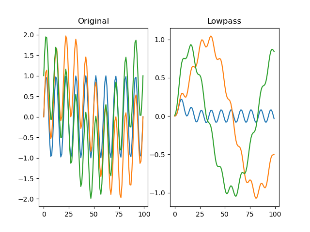
Arguments:
series-- A signal to filter.- Type: SeriesColumn
freq_max-- The maximum filter frequency.- Type: int
Keywords:
order-- The order of the filter.- Type: int
- Default: 2
sampling_freq-- The sampling frequence of the signal, orNoneto use the scipy default of 2 half-cycles per sample.- Type: int, None
- Default: None
Returns:
The filtered signal.
- Type: SeriesColumn
function interpolate(series)
Linearly interpolates missing (nan) data.
Example:
import numpy as np
from matplotlib import pyplot as plt
from datamatrix import DataMatrix, SeriesColumn, series as srs

LENGTH = 1 # Number of rows
DEPTH = 100 # Depth (or length) of SeriesColumns
MISSING = 50 # Nr of missing samples

# Create a sine wave with missing data
sinewave = np.sin(np.linspace(0, 2*np.pi, DEPTH))
sinewave[np.random.choice(np.arange(DEPTH), MISSING)] = np.nan
# And turns this into a DataMatrix
dm = DataMatrix(length=LENGTH)
dm.y = SeriesColumn(depth=DEPTH)
dm.y = sinewave
# Now interpolate the missing data!
dm.i = srs.interpolate(dm.y)

# And plot the original data as circles and the interpolated data as
# dotted lines
plt.clf()
plt.plot(dm.i.plottable, ':')
plt.plot(dm.y.plottable, 'o')
plt.show()
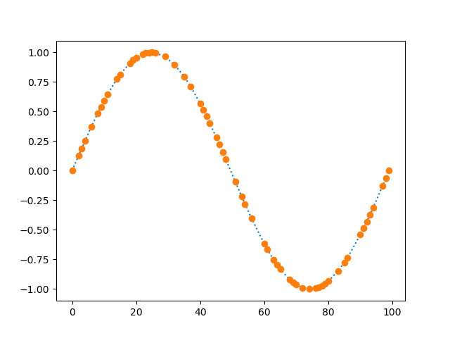
Arguments:
series-- A signal to interpolate.- Type: SeriesColumn
Returns:
The interpolated signal.
- Type: SeriesColumn
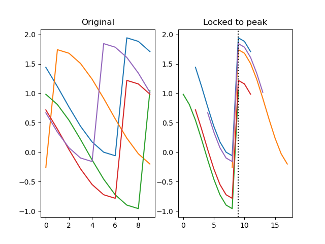
function lock(series, lock)
Shifts each row from a series by a certain number of steps along its depth. This is useful to lock, or align, a series based on a sequence of values.
Example:
import numpy as np
from matplotlib import pyplot as plt
from datamatrix import DataMatrix, SeriesColumn, series as srs

LENGTH = 5 # Number of rows
DEPTH = 10 # Depth (or length) of SeriesColumns

dm = DataMatrix(length=LENGTH)
# First create five traces with a partial cosinewave. Each row is
# offset slightly on the x and y axes
dm.y = SeriesColumn(depth=DEPTH)
dm.x_offset = -1
dm.y_offset = -1
for row in dm:
   row.x_offset = np.random.randint(0, DEPTH)
   row.y_offset = np.random.random()
   row.y = np.roll(
       np.cos(np.linspace(0, np.pi, DEPTH)),
       row.x_offset
   ) + row.y_offset
# Now use the x offset to lock the traces to the 0 point of the
# cosine, i.e. to their peaks.
dm.y2, zero_point = srs.lock(dm.y, lock=dm.x_offset)

plt.clf()
plt.subplot(121)
plt.title('Original')
plt.plot(dm.y.plottable)
plt.subplot(122)
plt.title('Locked to peak')
plt.plot(dm.y2.plottable)
plt.axvline(zero_point, color='black', linestyle=':')
plt.show()
Arguments:
series-- The signal to lock.- Type: SeriesColumn
lock-- A sequence of lock values with the same length as the Series. This can be a column, a list, a numpy array, etc.
Returns:
A (series, zero_point) tuple, in which series is a SeriesColumn and zero_point is the zero point to which the signal has been locked.
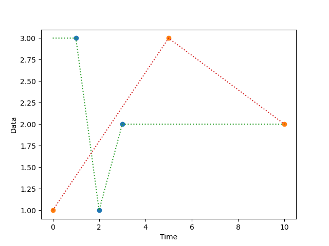
function normalize_time(dataseries, timeseries)
New in v0.7.0
Creates a new series in which a series of timestamps (timeseries) is
used as the indices for a series of data point (dataseries). This is
useful, for example, if you have a series of measurements and a
separate series of timestamps, and you want to combine the two.
The resulting series will generally contain a lot of nan values,
which you can interpolate with interpolate().
Example:
from matplotlib import pyplot as plt
from datamatrix import DataMatrix, SeriesColumn, series as srs, NAN

# Create a DataMatrix with one series column that contains samples
# and one series column that contains timestamps.
dm = DataMatrix(length=2)
dm.samples = SeriesColumn(depth=3)
dm.time = SeriesColumn(depth=3)
dm.samples[0] = 3, 1, 2
dm.time[0]    = 1, 2, 3
dm.samples[1] = 1, 3, 2
dm.time[1]    = 0, 5, 10
# Create a normalized column with samples spread out according to
# the timestamps, and also create an interpolate version of this
# column for smooth plotting.
dm.normalized = srs.normalize_time(
   dataseries=dm.samples,
   timeseries=dm.time
)
dm.interpolated = srs.interpolate(dm.normalized)
# And plot!
plt.clf()
plt.plot(dm.normalized.plottable, 'o')
plt.plot(dm.interpolated.plottable, ':')
plt.xlabel('Time')
plt.ylabel('Data')
plt.show()
Arguments:
dataseries-- A column with datapoints.- Type: SeriesColumn
timeseries-- A column with timestamps. This should be an increasing list of the same depth asdataseries. NAN values are allowed, but only at the end.- Type: SeriesColumn
Returns:
A new series in which the data points are spread according to the timestamps.
- Type: SeriesColumn
function reduce(series, operation=)
Transforms series to single values by applying an operation (typically a mean) to each series.
Version note: As of 0.11.0, the function has been renamed to
reduce(). The original reduce_() is deprecated.
Example:
import numpy as np
from datamatrix import DataMatrix, SeriesColumn, series as srs

LENGTH = 5 # Number of rows
DEPTH = 10 # Depth (or length) of SeriesColumns

dm = DataMatrix(length=LENGTH)
dm.y = SeriesColumn(depth=DEPTH)
dm.y = np.random.random( (LENGTH, DEPTH) )
dm.mean_y = srs.reduce(dm.y)

print(dm)
Output:
+---+---------------------+---------------------------------------------------+
| # |        mean_y       |                         y                         |
+---+---------------------+---------------------------------------------------+
| 0 |  0.4187258253638967 | [0.13613434 0.13418871 ... 0.13902066 0.56596511] |
| 1 | 0.44352492531855753 | [0.19814893 0.87787026 ... 0.1982677  0.71091438] |
| 2 |  0.5553004923181005 | [0.25517136 0.40037645 ... 0.73045827 0.30649484] |
| 3 |  0.5501859526863737 | [0.22379127 0.53499791 ... 0.97265194 0.18590858] |
| 4 |  0.4087578715889064 | [0.82124567 0.18695198 ... 0.52171991 0.07126145] |
+---+---------------------+---------------------------------------------------+
Arguments:
series-- The signal to reduce.- Type: SeriesColumn
Keywords:
operation-- The operation function to use for the reduction. This function should acceptseriesas first argument, andaxis=1as keyword argument.- Default:
- Default:
Returns:
A reduction of the signal.
- Type: FloatColumn
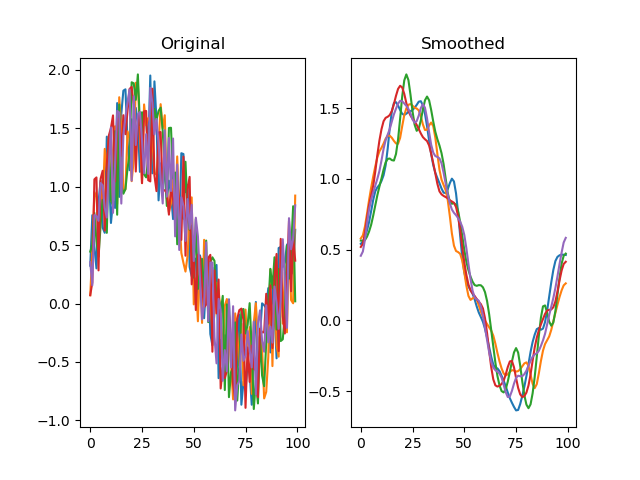
function smooth(series, winlen=11, wintype=u'hanning')
Smooths a signal using a window with requested size.
This method is based on the convolution of a scaled window with the signal. The signal is prepared by introducing reflected copies of the signal (with the window size) in both ends so that transient parts are minimized in the begining and end part of the output signal.
Adapted from:
Example:
import numpy as np
from matplotlib import pyplot as plt
from datamatrix import DataMatrix, SeriesColumn, series as srs

LENGTH = 5 # Number of rows
DEPTH = 100 # Depth (or length) of SeriesColumns

sinewave = np.sin(np.linspace(0, 2*np.pi, DEPTH))

dm = DataMatrix(length=LENGTH)
# First create five identical rows with a sinewave
dm.y = SeriesColumn(depth=DEPTH)
dm.y.setallrows(sinewave)
# And add a bit of random jitter
dm.y += np.random.random( (LENGTH, DEPTH) )
# Smooth the traces to reduce the jitter
dm.y2 = srs.smooth(dm.y)

plt.clf()
plt.subplot(121)
plt.title('Original')
plt.plot(dm.y.plottable)
plt.subplot(122)
plt.title('Smoothed')
plt.plot(dm.y2.plottable)
plt.show()
Arguments:
series-- A signal to smooth.- Type: SeriesColumn
Keywords:
winlen-- The width of the smoothing window. This should be an odd integer.- Type: int
- Default: 11
wintype-- The type of window from 'flat', 'hanning', 'hamming', 'bartlett', 'blackman'. A flat window produces a moving average smoothing.- Type: str
- Default: 'hanning'
Returns:
A smoothed signal.
- Type: SeriesColumn
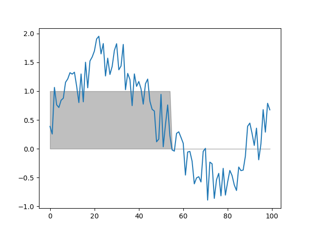
function threshold(series, fnc, min_length=1)
Finds samples that satisfy some threshold criterion for a given period.
Example:
import numpy as np
from matplotlib import pyplot as plt
from datamatrix import DataMatrix, SeriesColumn, series as srs

LENGTH = 1 # Number of rows
DEPTH = 100 # Depth (or length) of SeriesColumns

sinewave = np.sin(np.linspace(0, 2*np.pi, DEPTH))

dm = DataMatrix(length=LENGTH)
# First create five identical rows with a sinewave
dm.y = SeriesColumn(depth=DEPTH)
dm.y.setallrows(sinewave)
# And also a bit of random jitter
dm.y += np.random.random( (LENGTH, DEPTH) )
# Threshold the signal by > 0 for at least 10 samples
dm.t = srs.threshold(dm.y, fnc=lambda y: y > 0, min_length=10)

plt.clf()
# Mark the thresholded signal
plt.fill_between(np.arange(DEPTH), dm.t[0], color='black', alpha=.25)
plt.plot(dm.y.plottable)
print(dm)
plt.show()
Output:
+---+-------------------+---------------------------------------------------+
| # |         t         |                         y                         |
+---+-------------------+---------------------------------------------------+
| 0 | [1. 1. ... 0. 0.] | [0.3872822  0.25654575 ... 0.78936676 0.67559638] |
+---+-------------------+---------------------------------------------------+
Arguments:
series-- A signal to threshold.- Type: SeriesColumn
fnc-- A function that takes a single value and returns True if this value exceeds a threshold, and False otherwise.- Type: FunctionType
Keywords:
min_length-- The minimum number of samples for whichfncmust return True.- Type: int
- Default: 1
Returns:
A series where 0 indicates below threshold, and 1 indicates above threshold.
- Type: SeriesColumn
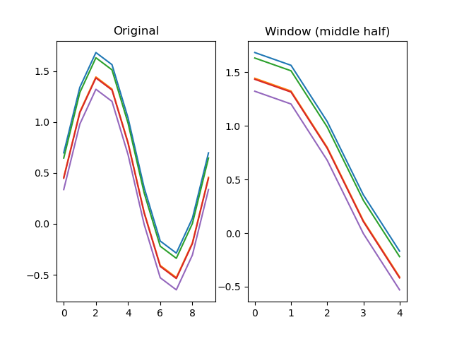
function window(series, start=0, end=None)
Extracts a window from a signal.
Version note: As of 0.9.4, the preferred way to get a window from a
series is with a slice: dm.s[:, start:end].
Example:
import numpy as np
from matplotlib import pyplot as plt
from datamatrix import DataMatrix, SeriesColumn, series as srs

LENGTH = 5 # Number of rows
DEPTH = 10 # Depth (or length) of SeriesColumns

sinewave = np.sin(np.linspace(0, 2*np.pi, DEPTH))

dm = DataMatrix(length=LENGTH)
# First create five identical rows with a sinewave
dm.y = SeriesColumn(depth=DEPTH)
dm.y.setallrows(sinewave)
# Add a random offset to the Y values
dm.y += np.random.random(LENGTH)
# Look only the middle half of the signal
dm.y2 = srs.window(dm.y, start=DEPTH//4, end=-DEPTH//4)

plt.clf()
plt.subplot(121)
plt.title('Original')
plt.plot(dm.y.plottable)
plt.subplot(122)
plt.title('Window (middle half)')
plt.plot(dm.y2.plottable)
plt.show()
Arguments:
series-- The signal to get a window from.- Type: SeriesColumn
Keywords:
start-- The window start.- Type: int
- Default: 0
end-- The window end, or None to go to the signal end.- Type: int, None
- Default: None
Returns:
A window of the signal.
- Type: SeriesColumn
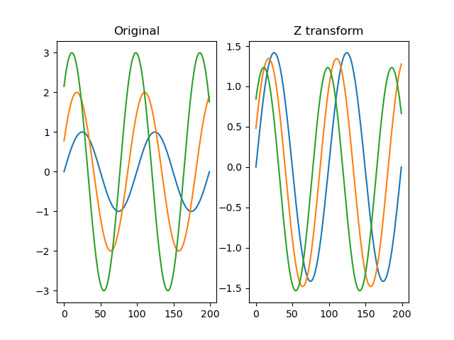
function z(series)
Applies a z-transform to the signal such that each trace has a mean value of 0 and a standard deviation of 1.
Example:
import numpy as np
from matplotlib import pyplot as plt
from datamatrix import DataMatrix, SeriesColumn, series as srs

LENGTH = 3
DEPTH = 200

# Create one fast oscillation, and two combined fast and slow
# oscillations
dm = DataMatrix(length=LENGTH)
dm.s = SeriesColumn(depth=DEPTH)
dm.s[0] = 1 * np.sin(np.linspace(0, 4 * np.pi, DEPTH))
dm.s[1] = 2 * np.sin(np.linspace(.4, 4.4 * np.pi, DEPTH))
dm.s[2] = 3 * np.sin(np.linspace(.8, 4.8 * np.pi, DEPTH))
dm.z = srs.z(dm.s)

# Plot the original signal
plt.clf()
plt.subplot(121)
plt.title('Original')
plt.plot(dm.s[0])
plt.plot(dm.s[1])
plt.plot(dm.s[2])
plt.subplot(122)
# And the filtered signal!
plt.title('Z transform')
plt.plot(dm.z[0])
plt.plot(dm.z[1])
plt.plot(dm.z[2])
plt.show()
Arguments:
series-- A signal to determine the z-transform for.- Type: SeriesColumn
Returns:
The z-transform of the signal.
- Type: SeriesColumn