


datamatrix.series
- What are series?
- function baseline(series, baseline, bl_start=-100, bl_end=None, reduce_fnc=None, method=u'divisive')
- function blinkreconstruct(series, vt=5, maxdur=500, margin=10, smooth_winlen=21, std_thr=3)
- function downsample(series, by, fnc=
) - function endlock(series)
- function reduce_(series, operation=
) - function smooth(series, winlen=11, wintype=u'hanning')
- function threshold(series, fnc, min_length=1)
- function window(series, start=0, end=None)
What are series?
A SeriesColumn is a column with a depth. For example, imagine a table that combines the names of two cities with their populations during the past four years. Here, the names the cities are single values that fit into a normal table. But the population corresponds to a series of values for each city. This is where the SeriesColumn comes in.
Example:
from matplotlib import pyplot as plt
from datamatrix import DataMatrix, SeriesColumn

NR_CITIES = 2
NR_YEARS = 4

dm = DataMatrix(length=NR_CITIES)
dm.city = 'Marseille', 'Lyon'
# Create a series for the population
dm.population = SeriesColumn(depth=NR_YEARS)
dm.population[0] = 850726, 850602, 851420, 797491 # Marseille
dm.population[1] = 484344, 479803, 474946, 445274 # Lyon
# Create a series for the years that correspond to the populations
dm.year = SeriesColumn(depth=NR_YEARS)
dm.year.setallrows( [2010, 2009, 2008, 1999])

print(dm)

plt.clf()
for row in dm:
    plt.plot(row.year, row.population, 'o-', label=row.city)
plt.legend(loc='upper left')
plt.xlabel('Year')
plt.ylabel('Population')
plt.xlim(1998, 2011)
plt.ylim(400000, 1000000)
plt.savefig('content/pages/img/series/series.png')
Output:
+---+-----------+---------------------------------------+-------------------------------+
| # |    city   |               population              |              year             |
+---+-----------+---------------------------------------+-------------------------------+
| 0 | Marseille | [ 850726.  850602.  851420.  797491.] | [ 2010.  2009.  2008.  1999.] |
| 1 |    Lyon   | [ 484344.  479803.  474946.  445274.] | [ 2010.  2009.  2008.  1999.] |
+---+-----------+---------------------------------------+-------------------------------+
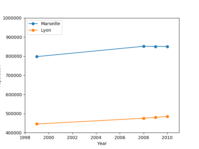
Figure 1. The populations of Marseille and Lyon over time.
Data of this kind is very common. For example, imagine a psychology experiment in which participants see positive or negative pictures, while their brain activity is recorded using electroencephalography (EEG). Here, picture type (positive or negative) is a single value that could be stored in a normal table. But EEG activity is a continuous signal, and could be stored as SeriesColumn.
function baseline(series, baseline, bl_start=-100, bl_end=None, reduce_fnc=None, method=u'divisive')
Applies a baseline to a signal
Example:
import numpy as np
from matplotlib import pyplot as plt
from datamatrix import DataMatrix, SeriesColumn, series

LENGTH = 5 # Number of rows
DEPTH = 10 # Depth (or length) of SeriesColumns

sinewave = np.sin(np.linspace(0, 2*np.pi, DEPTH))

dm = DataMatrix(length=LENGTH)
# First create five identical rows with a sinewave
dm.y = SeriesColumn(depth=DEPTH)
dm.y.setallrows(sinewave)
# Add a random offset to the Y values
dm.y += np.random.random(LENGTH)
# And also a bit of random jitter
dm.y += .2*np.random.random( (LENGTH, DEPTH) )
# Baseline-correct the traces, This will remove the vertical
# offset
dm.y2 = series.baseline(dm.y, dm.y, bl_start=0, bl_end=10,
       method='subtractive')

plt.clf()
plt.subplot(121)
plt.title('Original')
plt.plot(dm.y.plottable)
plt.subplot(122)
plt.title('Baseline corrected')
plt.plot(dm.y2.plottable)
plt.savefig('content/pages/img/series/baseline.png')
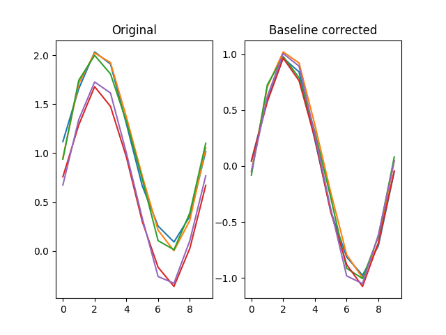
Figure 2.
Arguments:
series-- The signal to apply a baseline to.- Type: SeriesColumn
baseline-- The signal to use as a baseline to.- Type: SeriesColumn
Keywords:
bl_start-- The start of the window frombaselineto use.- Type: int
- Default: -100
bl_end-- The end of the window frombaselineto use, or None to go to the end.- Type: int, None
- Default: None
reduce_fnc-- The function to reduce the baseline epoch to a single value. If None, np.nanmedian() is used.- Type: FunctionType, None
- Default: None
method-- Specifies whether divisive or subtrace correction should be used. Divisive is the default for historical purposes, but subtractive is generally preferred.- Type: str
- Default: 'divisive'
Returns:
A baseline-correct version of the signal.
function blinkreconstruct(series, vt=5, maxdur=500, margin=10, smooth_winlen=21, std_thr=3)
Reconstructs pupil size during blinks. This algorithm has been designed and tested largely with the EyeLink 1000 eye tracker.
Source:
- Mathot, S. (2013). A simple way to reconstruct pupil size during eye blinks. http://doi.org/10.6084/m9.figshare.688002
Arguments:
series-- A signal to reconstruct.- Type: SeriesColumn
Keywords:
vt-- A pupil velocity threshold. Lower tresholds more easily trigger blinks.- Type: int, float
- Default: 5
maxdur-- The maximum duration (in samples) for a blink. Longer blinks are not reconstructed.- Type: int
- Default: 500
margin-- The margin to take around missing data.- Type: int
- Default: 10
smooth_winlen-- No description- Default: 21
std_thr-- No description- Default: 3
Returns:
A reconstructed singal.
- Type: SeriesColumn
function downsample(series, by, fnc=)
Downsamples a series by a factor, so that it becomes 'by' times shorter. The depth of the downsampled series is the highest multiple of the depth of the original series divided by 'by'. For example, downsampling a series with a depth of 10 by 3 results in a depth of 3.
Example:
import numpy as np
from matplotlib import pyplot as plt
from datamatrix import DataMatrix, SeriesColumn, series

LENGTH = 1 # Number of rows
DEPTH = 100 # Depth (or length) of SeriesColumns

sinewave = np.sin(np.linspace(0, 2*np.pi, DEPTH))

dm = DataMatrix(length=LENGTH)
dm.y = SeriesColumn(depth=DEPTH)
dm.y.setallrows(sinewave)
dm.y2 = series.downsample(dm.y, by=10)

plt.clf()
plt.subplot(121)
plt.title('Original')
plt.plot(dm.y.plottable, 'o-')
plt.subplot(122)
plt.title('Downsampled')
plt.plot(dm.y2.plottable, 'o-')
plt.savefig('content/pages/img/series/downsample.png')
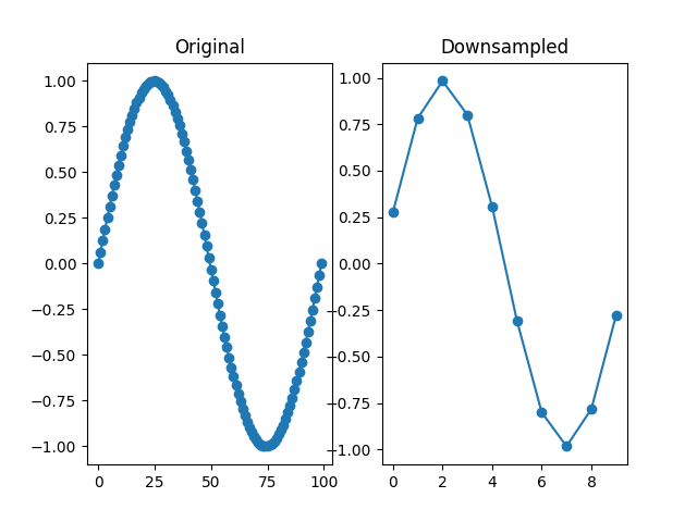
Figure 3.
Arguments:
series-- No descriptionby-- The downsampling factor.- Type: int
Keywords:
fnc-- The function to average the samples that are combined into 1 value. Typically an average or a median.- Type: callable
- Default:
Returns:
A downsampled series.
- Type: SeriesColumn
function endlock(series)
Locks a series to the end, so that any nan-values that were at the end are moved to the start.
Example:
import numpy as np
from matplotlib import pyplot as plt
from datamatrix import DataMatrix, SeriesColumn, series

LENGTH = 5 # Number of rows
DEPTH = 10 # Depth (or length) of SeriesColumns

sinewave = np.sin(np.linspace(0, 2*np.pi, DEPTH))

dm = DataMatrix(length=LENGTH)
# First create five identical rows with a sinewave
dm.y = SeriesColumn(depth=DEPTH)
dm.y.setallrows(sinewave)
# Add a random offset to the Y values
dm.y += np.random.random(LENGTH)
# Set some observations at the end to nan
for i, row in enumerate(dm):
       row.y[-i:] = np.nan
# Lock the degraded traces to the end, so that all nans
# now come at the start of the trace
dm.y2 = series.endlock(dm.y)

plt.clf()
plt.subplot(121)
plt.title('Original (nans at end)')
plt.plot(dm.y.plottable)
plt.subplot(122)
plt.title('Endlocked (nans at start)')
plt.plot(dm.y2.plottable)
plt.savefig('content/pages/img/series/endlock.png')
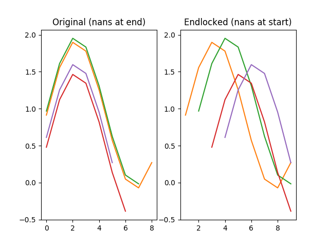
Figure 4.
Arguments:
series-- The signal to end-lock.- Type: SeriesColumn
Returns:
An end-locked signal.
- Type: SeriesColumn
function reduce_(series, operation=)
Transforms series to single values by applying an operation (typically a mean) to each series.
Example:
import numpy as np
from datamatrix import DataMatrix, SeriesColumn, series

LENGTH = 5 # Number of rows
DEPTH = 10 # Depth (or length) of SeriesColumns

dm = DataMatrix(length=LENGTH)
dm.y = SeriesColumn(depth=DEPTH)
dm.y = np.random.random( (LENGTH, DEPTH) )
dm.mean_y = series.reduce_(dm.y)

print(dm)
Output:
+---+-------------------------------------------------------+----------------+
| # |                           y                           |     mean_y     |
+---+-------------------------------------------------------+----------------+
| 0 | [ 0.59847021  0.98093191 ...  0.07659105  0.97542883] | 0.489982337067 |
| 1 | [ 0.77826279  0.5901201  ...  0.47342449  0.78378227] | 0.35278246037  |
| 2 | [ 0.59425941  0.96618109 ...  0.28001047  0.396487  ] | 0.555924142771 |
| 3 | [ 0.29879887  0.98810989 ...  0.88833685  0.62285926] | 0.626790759877 |
| 4 | [ 0.55612662  0.93839702 ...  0.28007682  0.68862264] | 0.526500980859 |
+---+-------------------------------------------------------+----------------+
Arguments:
series-- The signal to reduce.- Type: SeriesColumn
Keywords:
operation-- The operation function to use for the reduction. This function should acceptseriesas first argument, andaxis=1as keyword argument.- Default:
- Default:
Returns:
A reduction of the signal.
- Type: FloatColumn
function smooth(series, winlen=11, wintype=u'hanning')
Smooths a signal using a window with requested size.
This method is based on the convolution of a scaled window with the signal. The signal is prepared by introducing reflected copies of the signal (with the window size) in both ends so that transient parts are minimized in the begining and end part of the output signal.
Adapted from:
Example:
import numpy as np
from matplotlib import pyplot as plt
from datamatrix import DataMatrix, SeriesColumn, series

LENGTH = 5 # Number of rows
DEPTH = 100 # Depth (or length) of SeriesColumns

sinewave = np.sin(np.linspace(0, 2*np.pi, DEPTH))

dm = DataMatrix(length=LENGTH)
# First create five identical rows with a sinewave
dm.y = SeriesColumn(depth=DEPTH)
dm.y.setallrows(sinewave)
# And add a bit of random jitter
dm.y += np.random.random( (LENGTH, DEPTH) )
# Smooth the traces to reduce the jitter
dm.y2 = series.smooth(dm.y)

plt.clf()
plt.subplot(121)
plt.title('Original')
plt.plot(dm.y.plottable)
plt.subplot(122)
plt.title('Smoothed')
plt.plot(dm.y2.plottable)
plt.savefig('content/pages/img/series/smooth.png')
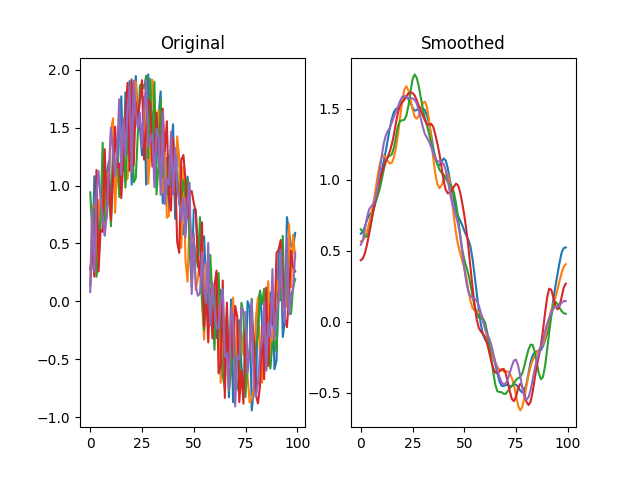
Figure 5.
Arguments:
series-- A signal to smooth.- Type: SeriesColumn
Keywords:
winlen-- The width of the smoothing window. This should be an odd integer.- Type: int
- Default: 11
wintype-- The type of window from 'flat', 'hanning', 'hamming', 'bartlett', 'blackman'. A flat window produces a moving average smoothing.- Type: str
- Default: 'hanning'
Returns:
A smoothed signal.
- Type: SeriesColumn
function threshold(series, fnc, min_length=1)
Finds samples that satisfy some threshold criterion for a given period.
Example:
import numpy as np
from matplotlib import pyplot as plt
from datamatrix import DataMatrix, SeriesColumn, series

LENGTH = 1 # Number of rows
DEPTH = 100 # Depth (or length) of SeriesColumns

sinewave = np.sin(np.linspace(0, 2*np.pi, DEPTH))

dm = DataMatrix(length=LENGTH)
# First create five identical rows with a sinewave
dm.y = SeriesColumn(depth=DEPTH)
dm.y.setallrows(sinewave)
# And also a bit of random jitter
dm.y += np.random.random( (LENGTH, DEPTH) )
# Threshold the signal by > 0 for at least 10 samples
dm.t = series.threshold(dm.y, fnc=lambda y: y > 0, min_length=10)

plt.clf()
# Mark the thresholded signal
plt.fill_between(np.arange(DEPTH), dm.t[0], color='black', alpha=.25)
plt.plot(dm.y.plottable)
plt.savefig('content/pages/img/series/threshold.png')

print(dm)
Output:
+---+-------------------------------------------------------+-----------------------+
| # |                           y                           |           t           |
+---+-------------------------------------------------------+-----------------------+
| 0 | [ 0.6515001   0.10468727 ...  0.21100606  0.48754461] | [ 1.  1. ...  0.  0.] |
+---+-------------------------------------------------------+-----------------------+
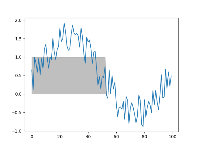
Figure 6.
Arguments:
series-- A signal to threshold.- Type: SeriesColumn
fnc-- A function that takes a single value and returns True if this value exceeds a threshold, and False otherwise.- Type: FunctionType
Keywords:
min_length-- The minimum number of samples for whichfncmust return True.- Type: int
- Default: 1
Returns:
A series where 0 indicates below threshold, and 1 indicates above threshold.
- Type: SeriesColumn
function window(series, start=0, end=None)
Extracts a window from a signal.
Example:
import numpy as np
from matplotlib import pyplot as plt
from datamatrix import DataMatrix, SeriesColumn, series

LENGTH = 5 # Number of rows
DEPTH = 10 # Depth (or length) of SeriesColumnsplt.show()

sinewave = np.sin(np.linspace(0, 2*np.pi, DEPTH))

dm = DataMatrix(length=LENGTH)
# First create five identical rows with a sinewave
dm.y = SeriesColumn(depth=DEPTH)
dm.y.setallrows(sinewave)
# Add a random offset to the Y values
dm.y += np.random.random(LENGTH)
# Look only the middle half of the signal
dm.y2 = series.window(dm.y, start=DEPTH//4, end=-DEPTH//4)

plt.clf()
plt.subplot(121)
plt.title('Original')
plt.plot(dm.y.plottable)
plt.subplot(122)
plt.title('Window (middle half)')
plt.plot(dm.y2.plottable)
plt.savefig('content/pages/img/series/window.png')
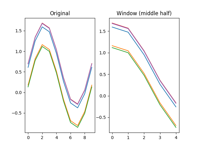
Figure 7.
Arguments:
series-- The signal to get a window from.- Type: SeriesColumn
Keywords:
start-- The window start.- Type: int
- Default: 0
end-- The window end, or None to go to the signal end.- Type: int, None
- Default: None
Returns:
A window of the signal.
- Type: SeriesColumn